Advanced Features
Cell Highlights
- FormulaChop looks for certain functions and highlights the cells in their precedent ranges that contribute to their results.

A dark outline shows highlighted cells
Tip
Any time a cell is highlighted, the label for its range becomes a link to only the highlighted cells
This can be very useful to focus on only the cells that are relevant to a calculation
Example
Navigate to the ‘Examples’ tab of this file to try the examples below for yourself
INDEX()
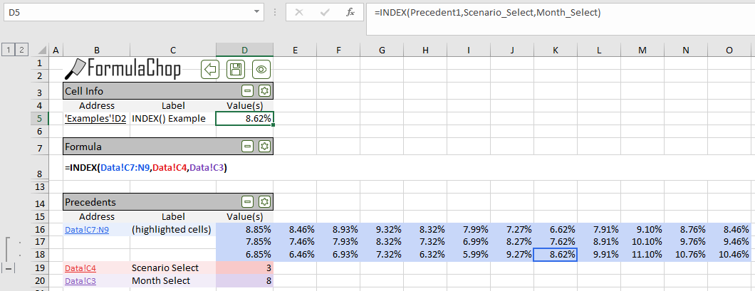
FormulaChop highlights the cell(s) returned by the INDEX() function
LOOKUP()
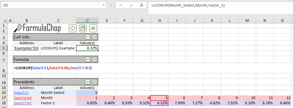
FormulaChop highlights the cell(s) in which the search value is found, as well as the return value.
- This works for
LOOKUP(),HLOOKUP()andVLOOKUP()
CHOOSE()
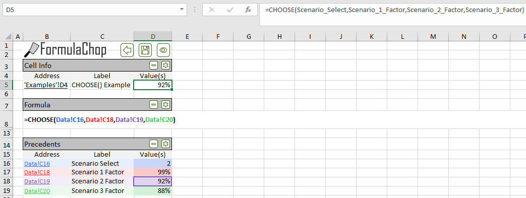
FormulaChop highlights cell(s) returned by CHOOSE()
SUMIF(), COUNTIF(), AVERAGEIF()
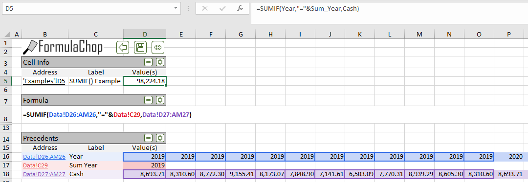
FormulaChop highlights the cell(s) where the condition is true, as well as the cell(s) being summed/counted/averaged
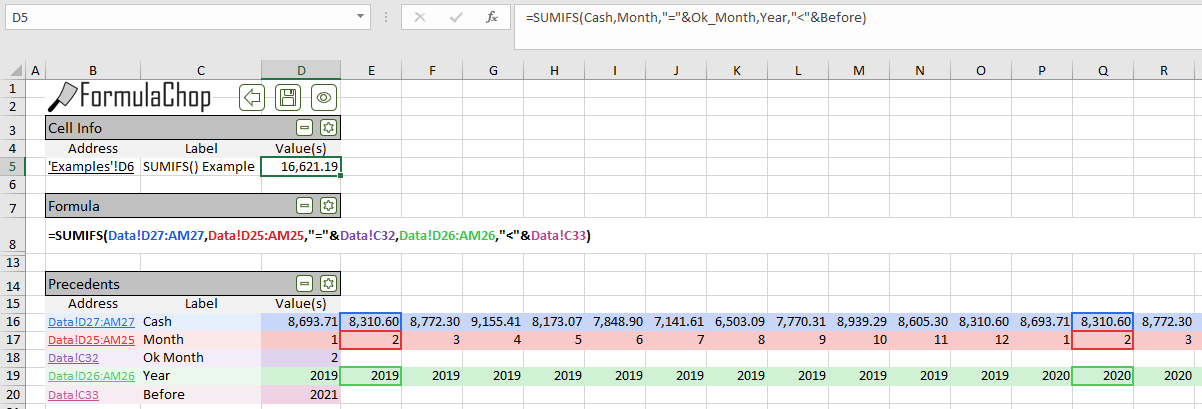
This works for the plural versions of these functions: SUMIFS() and COUNITFS()
MATCH()
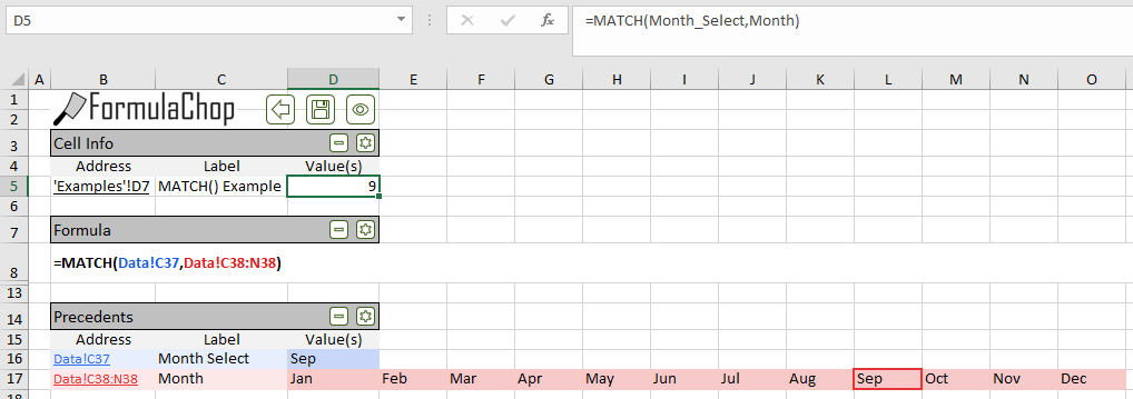
FormulaChop highlights matching cell(s)
Advanced Formulas
- FormulaChop supports advanced formula constructions which are used in large, complex spreadsheets.
Example
See this file to try the examples below for yourself
Formulas Which Return Ranges
- Formulas can be written such that they return a range, instead of a single value.
- In this situation, Excel will pick the value in the returned range that aligns with the calling cell.
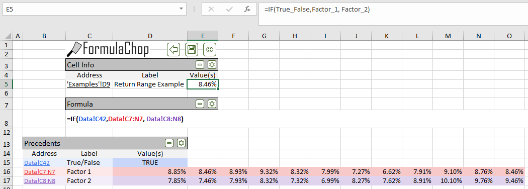
FormulaChop handling a formula which returns a range
Example:
The figure above shows FormulaChop output from cell D9. The chopped formula is:
=IF(True_False,Factor_1, Factor_2)
This IF() statement returns a range of cells, depending on the value in True_False.
Excel uses the relative alignment of the calling cell, G3 and the returned range, Factor_1 (F7:Q7), to decide which value to in the returned range to show.
Because the calling cell is in column G, the value in column G of the range Factor_1 will be returned
FormulaChop recognizes this situation and recreates all the ranges’ alignment on the FormulaChop Tab.
- A common example of this situation is the use of
INDEX()with a0argument. - When
0is given as an argument for a row or column,INDEX()returns the entire row or column. - Because
INDEX()is returning a range, Excel will use the relative alignment of the calling cell and the resulting range to give the formula’s single result
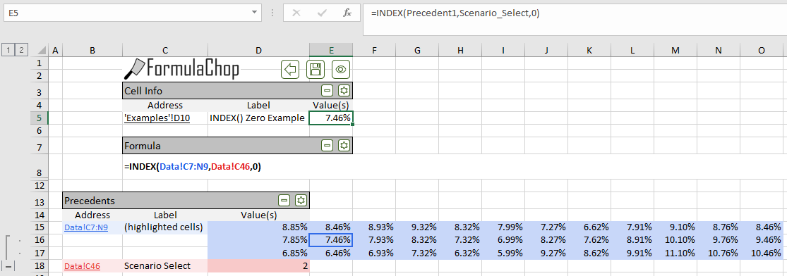
FormulaChop handling INDEX() Zero Argument
Example
The figure above shows FormulaChop output from cell D10. The chopped formula is:
=INDEX(Precedent1,Scenario_Select,0)
Instead of specifying a column, this formula uses 0 as its column argument.
Because the cell containing this formula is in column G, INDEX() will use column G in the range Precedent1 (F6:Q8).
This feature also applies when the calling cell is on a different tab from the range in the first argument to INDEX().
OFFSET()
- Unique among all Excel functions, the
OFFSET()function is able to depend on ranges without explicitly referring to them.
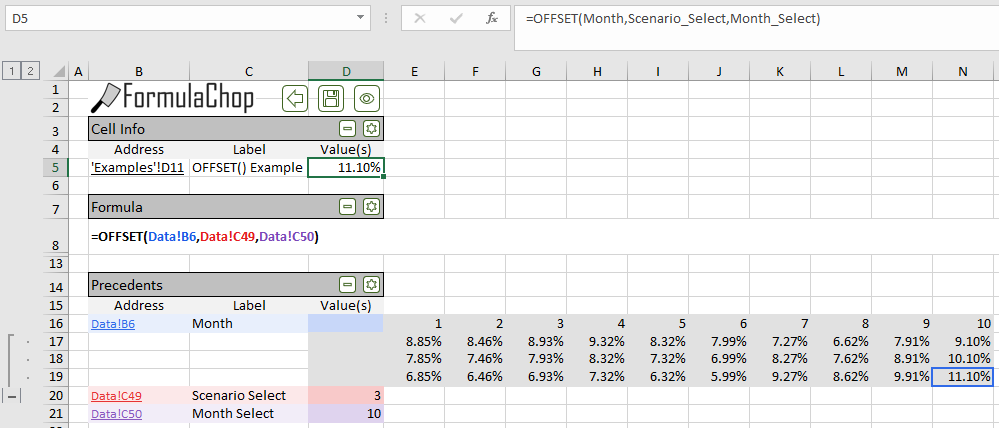
FormulaChop handling an OFFSET() function
- FormulaChop evaluates each
OFFSET()in the formula, and determines the range it is referring to, and copies that range to the FormulaChop Tab
INDIRECT()
- The
INDIRECT()function accepts as text the address of a range in the workbook, then it returns that range.
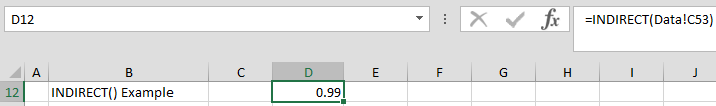
A formula using the INDIRECT() function
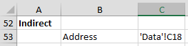
The cell referenced by the INDIRECT() function: Data!C50. Notice it contains a cell address as text.
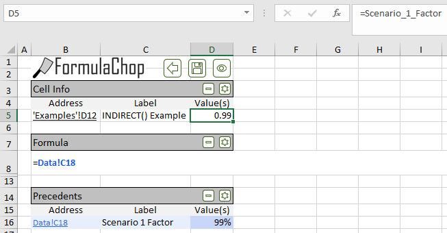
FormulaChop handling an INDIRECT() function. The INDIRECT() function has been replaced by its result: Data!C18.
- FormulaChop evaluates each call to
INDIRECT()and finds its resulting range - Then FormulaChop replaces the call to
INDIRECT()in the formula with the range - The range returned by
INDIRECT()appears on the FormulaChop Tab
Dynamic Ranges
- Excel allows two functions,
OFFSET()andINDEX(), to be used in the place of a cell when defining a range
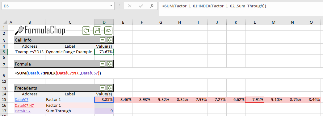
FormulaChop handling a Dynamic Range.
Example
The figure above shows FormulaChop output from cell D12. The chopped formula is:
=SUM(Factor_1_01:INDEX(Factor_1_02,,Sum_Through))
The value of
Sum_Through(F11) is9Factor_1_01is the rangeB10,Factor_1_02is the rangeB10:M10INDEX(Factor_1_02,,Sum_Through)will return the cellJ10B10+9columns =J10
Now, the formula reads
SUM(B10:J10)
The value in Sum_Through defines the size of the range being summed. This is what makes the range “dynamic”
- FormulaChop is able to handle Dynamic Ranges by only showing a single range on the FormulaChop Tab
- The start and end of the Dynamic Range is highlighted
3D Ranges
- Excel allows ranges to be defined across many tabs. This is called a 3D Range.
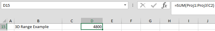
A formula with a 3D range. Notice the range of tabs specified: Proj1:Proj3.
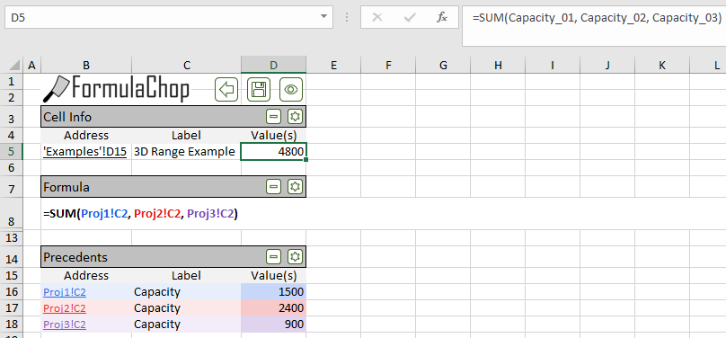
FormulaChop handling a 3D Range. Notice the 3D range has been replaced with a list of ranges.
Example
The figure above shows FormulaChop output from a cell using a 3D Range. This workbook has tabs Proj1, Proj2 and Proj3.
Each of these tabs has the same layout, with a “Capacity” value in cell C2. The chopped formula is:
=SUM('Proj1:Proj3'!C2)
This formula sums the values in cell C2 in all of the tabs between Proj1 and Proj3.
- FormulaChop looks for 3D ranges in the formula, and replaces them with a comma-separated list of ranges on each tab
Labels
FormulaChop does its best to automatically find the labels for the ranges in the Precedents and Dependents sections
FormulaChop will look for labels
- Horizontally if the range is a row (determined by the Orientation setting)
- Vertically if the range is a column (determined by the Orientation setting)
- In the direction set by the Orientation setting if the range is a single cell. Then in the other direction if no label is found.
The start and direction of the search depends on the setting of Label Search Direction
- Out<-Inside The search starts from the first cell in the precedent and steps outward
- Outside->In The search starts from the first row/column of the worksheet and steps inward
If FormulaChop finds a cell containing text, and the text meets some criteria, FormulaChop decides that the text is the label
Ranges that are blocks (i.e. have more than 2 rows and columns) are only labelled if they are named ranges
Label Criteria
While FormulaChop is looking for a label, it will skip a cell if:
- Cell does not contain text
- Cell is empty or blank
- Text is fewer than 3 characters long
- Text is surrounded by parentheses or brackets (e.g. “(kWh)” and “[kWh]” would not be considered labels)
- Text is “USD”
Custom Criteria
You may specify your own text for FormulaChop to ignore while searching for labels
FormulaChop will look for a Named Range named fcIgnoreText
- Any text inside
fcIgnoreTextwill be ignored when FormulaChop searches for labels - This range may be any shape or size, and may be on any tab
- Locating
fcIgnoreTexton the FormulaChop Tab is not recommended
Rules for Turning Labels into Range Names
FormulaChop follows these rules when labels are being used to name precedent ranges
- Characters which are invalid in Named Ranges will be replaced with an underscore (“_”)
Example
A range with the label “Special Expenses ($)” would be named “Special_Expenses____”
A range with the label “11th” would be named “_1th”
- Leading underscores will be removed if possible
Example
A range with the label “(-) Cash Distributions” would be named “Cash_Distributions”
A range with the label “101st” would be named “_01st”
- Repeat names will be numbered
Example
Two ranges with the label “date” would be named “date_01” and “date_02”
- Labels which could be interpreted as cell addresses will not be labelled
Example
A range with the label “P50” will not be named, because “P50” is the address of a cell
- Ranges with no label are named “PrecedentX”, where X is position in the order of appearance in the formula
Example
A range with no label, which appears 3rd in the formula, would be named “Precedent3”
Unsupported Functions
FormulaChop is unable to support some Excel functions. FormulaChop will not run on formulas which contain these functions.
- In general, this is because these functions rely on aspects of the precedents cells which cannot be copied to the FormulaChop Tab
- For example, the
ROW()function returns the row number of its argument- FormulaChop rebuilds the formula on the FormulaChop Tab, and would be unable to always place the precedent cells in the same row as the chopped formula
Unsupported Function List
CELL()COLUMN()FILTER()FORMULATEXT()ROW()SINGLE()SORT()TRANSPOSE()UNIQUE()
Array Formulas
FormulaChop is unable to support Array Formulas.
- Because FormulaChop is designed to only be run on one formula in one cell, it is unable to copy an array of cells to the FormulaChop Tab
INDIRECT() Array Output
FormulaChop is unable to support formulas which use an INDIRECT() function that returns an array of ranges. In this context, there is no way to replace the INDIRECT() function with an ordinary range.
Please see this SuperUser post to know more about this issue.
Deleting The FormulaChop Tab
- The FormulaChop Tab is automatically deleted before the spreadsheet is saved or closed
- Any tabs which were saved using the Save command (or renamed manually) will not be deleted
- Running FormulaChop will not require the spreadsheet to be saved unless:
- It needed to be saved before FormulaChop was run
- Calculating the spreadsheet (i.e. pressing
F9) causes it to require saving
FormulaChop History
- FormulaChop saves a history of cells which have been chopped
- To go back in the history, use
Ctrl + Shift + V(see Chop Commands) - To go forward in the history, use
Ctrl + Shift + F(see Chop Commands) - If you are back in the history and you chop a new cell, this cell will become the latest in the history